Power Purchase Agreement Financial Models

Introduction

Commercial and industrial energy buyers across India face a persistent challenge: grid tariffs are rising unpredictably, often escalating 5–7% annually, while most businesses sign long-term Power Purchase Agreements without rigorous financial analysis. The outcome is either significant overpayment or missed savings that compound over decades.

A PPA financial model is the analytical engine that separates a strategically sound energy deal from a costly 25-year mistake. With India's C&I renewable capacity projected to surge 40% to reach 57 GW by fiscal 2028 according to CRISIL Ratings, getting the financial model right determines whether a signed deal delivers savings or quietly erodes margins for two decades.

This guide unpacks the core components, output metrics, and India-specific regulatory inputs that determine whether a PPA creates value or destroys it. You'll learn how to:

• Structure cash flow projections across a 25-year agreement horizon
• Interpret IRR and DSCR benchmarks that lenders and developers actually use
• Stress-test assumptions through scenario analysis
• Navigate state-level charge structures that can shift landed power costs by ₹1–3 per kWh

TLDR

• PPA financial models project 15–25 years of revenue, costs, debt service, and returns to quantify deal viability
• Core inputs: plant capacity, energy yield (P50/P90), degradation, tariff structure, CAPEX/OPEX, and financing terms
• Equity IRR targets 16–20% for Indian hybrid projects, with payback periods of 6–8 years
• Lender benchmarks require DSCR of 1.25–1.40x minimum; NPV and LCOE confirm long-term cost competitiveness
• Stress-testing covers tariff escalation, generation shortfalls, regulatory shifts, and O&M inflation
• India-specific layers like open access charges, DISCOM tariff benchmarks, and state surcharges determine landed cost

What Is a PPA Financial Model?

A PPA financial model is a structured, multi-year cash flow projection—typically spanning 15–25 years—that quantifies the economic viability of a Power Purchase Agreement. It translates technical parameters (energy yield, degradation, resource variability) and commercial terms (tariff, escalation, charges) into financial outcomes guiding both developers and buyers.

Developer Perspective: Sizing Debt and Equity Returns

Developers use the model to size debt capacity, target equity IRR (typically 16–20% for hybrid projects per FinRaja), ensure DSCR covenants are met, and set a minimum viable tariff for competitive bidding. The cash flow waterfall follows a defined sequence:

• Gross revenue minus OPEX yields EBITDA
• EBITDA services senior debt obligations
• Reserve accounts are funded next
• Taxes are settled, with residual cash distributed to equity

C&I Buyer Perspective: Landing Cost vs. Grid Tariff

C&I buyers use the same framework differently — to compare the all-in landed cost of PPA power against current and projected grid tariffs. Open access renewable power typically delivers electricity at ₹2.5–4 per kWh, often below industrial grid rates.

For large energy consumers such as data centres, that gap translates to approximately ₹50 lakh per MW in annual savings (Fourth Partner Energy).

When to Build or Commission a Model

Large C&I consumers evaluating competing PPA offers need at least a buyer-side model to understand:

• True cost-of-power after all regulatory charges
• Payback on any upfront security deposit or commitment
• Protection against escalation risk over the contract term
• NPV of savings versus remaining on grid power

Building these models from scratch is time-consuming. Opten Power's platform automates this — delivering instant IRR, payback, and regulatory cost analysis across multiple developer offers so procurement teams can evaluate deals without maintaining complex spreadsheets.

Revenue and Energy Generation Inputs

The most consequential input in any PPA financial model is projected annual energy generation. Small errors compound over 25 years, turning profitable projects into stranded assets.

Installed Capacity and Energy Yield

Financial models start with the plant's installed capacity (MW or MWp) and expected annual energy yield, measured in full load hours or MWh per MWp. This figure is driven by location-specific resource data—solar irradiance for PV projects, wind resource assessments for wind farms.

Capacity Utilization Factor (CUF) measures how efficiently a plant generates energy relative to its theoretical maximum. India's hybrid projects deliver significantly higher CUF than standalone technologies:

Technology	Typical CUF Range
Standalone Solar PV	18–25%
Standalone Onshore Wind	22–35%
Wind-Solar Hybrid	35–50%

Source: IEEFA/JMK Research

The hybrid advantage stems from seasonal complementarity: India's monsoon months (June–September) produce 62% of total annual wind energy while solar output drops approximately 14% during the same period. Wind peaks at night and early morning; solar peaks midday.

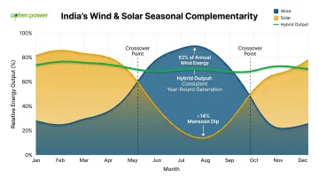
This means hybrid plants achieve roughly twice the energy output per MW of interconnection capacity compared to standalone solar, cutting fixed costs per unit of energy roughly in half.

Degradation Modeling

Solar PV modules degrade at approximately 0.5% per year. Over a 25-year PPA, this compounds to roughly 12% cumulative output reduction. Financial models must apply year-by-year degradation to base-year yield—a Year 1 plant generating 100 MWh will produce approximately 88 MWh in Year 25 from the same capacity.

That output decline directly affects revenue—which is why the tariff structure modeled alongside it must be equally precise.

PPA Tariff Structure and Escalation

Most C&I PPAs in India use a fixed per-kWh rate with annual escalation clauses of 1–3% (SunWave Tech). The structure typically includes:

• Base tariff: Fixed rate per unit consumed
• Escalation clause: Annual percentage increase (1–3% standard, or CPI-linked)
• Payment terms: Monthly billing based on metered generation

While SECI utility-scale tenders use flat tariffs, C&I contracts incorporate escalation to hedge developer costs.

The financial model must compound this escalation annually. A ₹4.00/kWh tariff with 3% escalation reaches ₹8.37/kWh by Year 25—so the choice of escalation rate has significant long-term revenue implications for both parties.

Seasonality, Availability, and Banking

Monthly or quarterly production profiles reflecting seasonal generation patterns are critical for accurate cash flow timing. Availability assumptions account for planned and unplanned downtime—standard assumptions run 95–98% for solar, 90–95% for wind.

Banking rules create additional complexity. Several states now restrict energy banking:

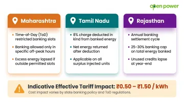
• Maharashtra: Time-of-day restricted banking slots
• Tamil Nadu: 8% banking charge in kind
• Rajasthan: Annual banking with 25–30% consumption caps for captive users

These charges must be modeled explicitly as operating cost line items, not rounded away—they can shift effective tariffs by ₹0.50–1.50 per kWh.

Cost Structure, Financing, and the Cash Flow Waterfall

Capital Expenditure Benchmarks

India achieved the lowest utility-scale solar installed cost globally in 2024 at USD 525/kW according to IRENA. Wind-solar hybrid projects range from ₹5.5–6.8 crore per MW depending on location and technology mix.

CAPEX includes:

• EPC costs (equipment, installation, testing)
• Grid connection and evacuation infrastructure
• Land acquisition or lease payments
• Development fees and contingency buffers

The distinction between turn-key EPC (fixed price, developer risk) and EPCM (cost-plus, buyer risk) directly affects cost certainty in the model.

Operational Expenditure

OPEX for hybrid projects runs at approximately 1.5–2.0% of CAPEX annually. Components include:

• Fixed: O&M contract fees, land lease, insurance, management charges
• Variable: Transmission and wheeling charges, scheduling fees, deviation penalties

OPEX should be modeled with appropriate escalators (typically 3–5% inflation-linked) rather than modeled flat. Co-located hybrid systems achieve approximately 7–8% lower costs than standalone solar due to shared infrastructure.

Debt Structure and Sizing

Project debt is sized either by:

• Maximum debt-to-capital ratio (typically 70:30 to 75:25 debt-to-equity)
• Minimum DSCR covenant (lenders require 1.20–1.40x for Indian renewables)

Sculpted debt schedules shape repayments to match project cash flow profiles and maintain DSCR above covenant thresholds throughout the tenor, rather than using linear repayment. That repayment structure feeds directly into how cash is distributed across stakeholders — which is where the waterfall becomes critical.

The Cash Flow Waterfall

The cascade of payments follows strict priority:

1. Gross Revenue (tariff × energy delivered)
2. Operating Costs (O&M, land lease, insurance)
3. EBITDA (Earnings Before Interest, Taxes, Depreciation, Amortization)
4. Debt Service (interest + principal)
5. Reserve Accounts (DSRA sized at 6 months forward debt service; MMRA for major component replacements)
6. Taxes (corporate tax, after deducting interest expense)
7. Free Cash Flow to Equity

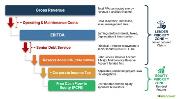
Lenders get paid before equity receives distributions — this priority ordering is what makes the project bankable to debt providers in the first place.

Tax and Depreciation Benefits

India's Income Tax Act provides two mechanisms that improve post-tax equity returns:

• 40% accelerated depreciation in Year 1 on renewable energy assets, reducing taxable income substantially in early project years
• Tax-deductible interest on debt, which lowers the effective tax burden and can shift project IRR by 200–400 basis points depending on leverage and corporate tax rates

Together, these mechanisms make higher-leverage structures more attractive for equity investors than the headline IRR figures suggest.

Key Financial Metrics in PPA Evaluation

Four metrics determine whether a PPA financial model signals "go" or "no-go."

Internal Rate of Return (IRR)

IRR is the discount rate that makes the project's NPV equal to zero. Two variants matter:

• Levered Equity IRR: Return to equity investors after debt service—what developers target
• Unlevered Project IRR: Pre-financing returns—useful for comparing across capital structures

For Indian hybrid wind-solar projects, benchmark ranges are:

Metric	Benchmark Range
Project IRR (Unlevered)	13–17%
Equity IRR (Levered)	16–20%

Source: FinRaja

The spread between project and equity IRR reflects leverage benefit: with 70:30 debt-to-equity ratios, financial leverage amplifies equity returns above project-level returns. IRR tells you the return story—but lenders care more about whether cash flows reliably cover debt obligations.

Net Present Value (NPV)

NPV measures the present value of future cash flows minus the initial investment at a required discount rate. A positive NPV confirms the project creates value at that return threshold.

For C&I buyers, the relevant calculation is more direct: take the difference between PPA landed cost and DISCOM tariff, multiply by annual consumed units, and discount that savings stream to present value across the 25-year term. That single figure converts a tariff comparison into a rupee-value business case.

Debt Service Coverage Ratio (DSCR)

DSCR = Cash Flow Available for Debt Service (CFADS) ÷ Total Debt Service in a period.

Indian renewable project lenders typically require minimum DSCR of 1.20x, with averages of 1.25–1.40x considered healthy. The model must demonstrate this ratio is maintained throughout the debt tenor, especially under conservative P90 production scenarios. A DSCR below covenant can trigger cash lock-up provisions or technical default.

DSCR defines the floor lenders will accept; LCOE then tells you whether the project's economics justify the tariff being offered.

Levelized Cost of Energy (LCOE)

LCOE divides total lifecycle costs (CAPEX plus discounted OPEX) by total lifetime energy output, producing a per-kWh cost you can compare directly against the PPA tariff or grid rate.

SECI auction-discovered tariffs provide market-validated benchmarks:

• Record low hybrid tariff: ₹2.34/kWh (Tranche IV) (Mercom India)
• Recent hybrid range: ₹3.43–3.46/kWh (Tranche VIII) (SECI Results)

A project LCOE below the offered PPA rate leaves pricing margin for the developer. An LCOE above grid tariff makes the economics unworkable for the buyer.

Payback Period and C&I Savings

Simple payback measures time to recover any upfront commitment (security deposit, equity investment). For hybrid projects, key benchmarks are:

• Payback period typically falls between 6–8 years
• Equity investors receive free cash flow for the remaining 17–19 years of the project life
• C&I buyers measure value through total NPV of savings, not payback alone

A real-world example grounds this: CleanMax's 32.5 MW hybrid project for NTT in Karnataka delivers power at 40–50% below prevailing grid tariff, with projected lifetime savings of ₹523 crore over 25 years (JMK Research).

Running these five metrics across competing developer offers — landed cost, IRR, DSCR, LCOE, and payback — simultaneously is where platforms like Opten Power replace weeks of spreadsheet work with real-time comparison across live project listings.

Scenario Analysis and Risk Sensitivity in PPA Models

A single base-case model is insufficient when projecting 15–25 years into an uncertain future. Robust PPA financial models employ scenario analysis and sensitivity testing to bracket outcomes and identify risk factors requiring contractual protection.

Standard Scenario Framework

Best practice employs three core scenarios:

• Base Case: P50 energy yield, expected tariff escalation, typical O&M inflation, current regulatory charges
• Upside Case: Higher grid tariff escalation widening the savings gap, favorable regulatory outcomes (lower open access charges), full availability
• Downside Case: P90 energy yield (typically 4–10% below P50), adverse regulatory changes (CSS increases, banking charge introductions), higher O&M and transmission charge escalation

The P90 downside scenario must still demonstrate DSCR above covenant thresholds for the project to be bankable. Lenders size debt against P90 projections while equity returns are modeled on P50.

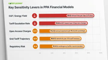
Key Sensitivity Levers

Five variables drive the widest range of financial outcomes:

Sensitivity Variable	Risk Direction	Indicative Impact
CUF / Energy Yield	Downside if below P50	1 pp CUF drop on a 100 MW project at ₹3.50/kWh = ~₹3 crore annual revenue loss
Tariff Escalation Rate	Both directions	1% vs. 3% annual escalation doubles nominal tariff by Year 25 at the higher rate
Open Access Charges	Downside	State-level charges shift landed cost by ₹1–3/kWh — the same project can be viable in one state, uneconomic in another
Grid Tariff Trajectory	Downside if grid stagnates	If grid tariffs flatten while PPA costs escalate 3% annually, buyer savings compress over time
Regulatory Risk	Downside	Banking rule changes, CSS increases, or ISTS waiver withdrawals can shift project economics mid-contract

Contingency and Risk Buffers

Lenders require reserve accounts reflected in the model:

• Debt Service Reserve Account (DSRA): Sized at 6 months forward debt service as standard liquidity cushion
• Major Maintenance Reserve Account (MMRA): Funds periodic equipment replacements (inverters, transformer overhauls) outside routine O&M

Both reserves are funded from operating cash flow before equity distributions. This depresses early-year equity returns — but without them, the project won't clear lender bankability checks regardless of how strong the base-case IRR looks.

India-Specific Modeling Considerations for C&I Buyers

India's electricity regulation is a concurrent subject, creating significant inter-state variation in charges, procedures, and risk profiles. The financial viability of a C&I open access PPA depends as much on state-level regulatory variables as on project-level technical parameters.

Open Access Charges and Landed Cost

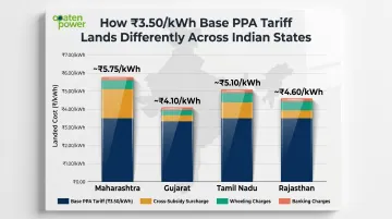
In India, C&I buyers procuring power through open access incur multiple charges that vary dramatically by state:

Charge Component	Maharashtra	Tamil Nadu	Gujarat	Rajasthan
Cross-Subsidy Surcharge	₹1.36–2.92/kWh	Capped at 20% of tariff	Exempt (captive)	Per RERC order
Wheeling Charges	₹0.48–0.60/kWh	₹1.04/kWh (HT)	50% exempt (captive)	Per RERC order
Banking	ToD-restricted slots	8% in kind	₹1.50/kWh	Annual, 25–30% cap
BESS Mandate	No	No	No	5% capacity, 2hr min

Sources: MSEDCL; TNERC; Gujarat Policy; RERC

These charges can amount to 30–50% of the base PPA tariff and must be modeled explicitly. A ₹3.50/kWh PPA in Maharashtra might land at ₹5.50–6.00/kWh after all charges, while the same PPA in Gujarat under group captive structure could land at ₹4.00–4.20/kWh.

DISCOM Benchmark Tariff as Comparison Baseline

The model's savings calculation depends on current and projected DISCOM tariff. Industrial tariffs vary significantly:

• High-tariff states (Maharashtra, Delhi, Tamil Nadu): ₹7–12/kWh
• Moderate-tariff states (Gujarat, Rajasthan, Karnataka): ₹5–8/kWh
• Lower-tariff states (Punjab, Madhya Pradesh): ₹4–6/kWh

Projecting future grid tariff escalation—historically 3–7% for industrial consumers—is typically where the savings case is strongest. Opten Power's Real-Time DISCOM Intelligence aggregates standardized landing prices across all 16+ states, removing the need to cross-reference individual state regulatory commission orders for benchmarking.

Regulatory and Contractual Risk Inputs

Four India-specific regulatory scenarios warrant explicit stress-testing in the model:

1. Banking rules differ materially by state — Maharashtra restricts banking to time-of-day slots, Tamil Nadu charges 8% in kind, and Rajasthan mandates BESS for RE projects over 5 MW. Model each state's banking charges as a separate line item.

2. DSM tolerance tightening: CERC narrowed deviation bands for solar/hybrid from ±10% to ±5% effective April 2026 (CERC Order). Budget for either improved forecasting costs or higher penalty exposure.

3. ISTS waiver phase-out: Projects with COD between July 2025–June 2026 pay 25% of applicable ISTS charges, stepping up to 100% by July 2028 (CERC Order). Commissioning delays create direct tariff risk that must be reflected in sensitivity runs.

4. DISCOM payment delays: Renewable projects hold "must-run" status with 100% minimum generation compensation for curtailment (SECI PSA), but payment timelines vary by state DISCOM health. Model this as a cash flow timing risk, not just a default risk.

Global PPA templates don't capture these variables by default — India-specific models need dedicated inputs for each.

Frequently Asked Questions

What is PPA in finance?

A Power Purchase Agreement (PPA) in finance is a long-term contractual arrangement between a power generator and a buyer for the sale of electricity at a pre-agreed price. In project finance, it serves as the primary revenue contract that enables developers to raise debt and structure returns over the asset's operational life.

What are best practices for structuring financial data in Excel for a PPA model?

Separate input sheets (time-independent assumptions and time-dependent schedules) from calculation and output sheets. Use named ranges and scenario switches for flexibility. Avoid hardcoded numbers in formulas—all constants should reference clearly labeled input cells to ensure the model can be audited and updated easily.

What is a good IRR for a renewable energy PPA project in India?

Equity IRR expectations for Indian renewable projects typically range from 16–20% for hybrid wind-solar configurations, with unlevered project IRR of 13–17% (FinRaja). Levered IRR exceeds unlevered IRR because interest deductions reduce tax liability and debt magnifies returns when project yields outpace borrowing costs.

What is DSCR and why does it matter in PPA project financing?

DSCR (Debt Service Coverage Ratio) measures cash flow available for debt service divided by total debt service (principal plus interest). Lenders use it to size and covenant project debt—minimum DSCR of 1.20–1.40x is standard for Indian renewable projects. A DSCR below the covenant threshold can trigger cash lock-up provisions or technical default, cutting off equity distributions.

How do C&I buyers evaluate whether a PPA is financially better than grid power?

The core comparison is the PPA's effective landed cost (base tariff plus open access charges, banking fees, wheeling losses) versus the DISCOM tariff over the contract life. NPV of savings—calculated as the tariff differential across consumed units discounted to present value—and payback period are the primary decision metrics.

What is the difference between a physical PPA and a virtual PPA from a financial modeling perspective?

In a physical PPA, the buyer pays the generator directly for delivered electricity, and the cost flows through operating expenses with actual energy delivered via open access. In a virtual (financial/synthetic) PPA, only the financial settlement of the price difference flows through P&L, and the buyer continues purchasing power from the grid—making the physical and financial flows entirely separate.